But if the VLOOKUP formula can’t find the information that it is looking for, it will display an error in the form of #N/A. This can be problematic, especially if the appearance of your data is important. Fortunately, you can make a minor alteration to your VLOOKUP formula to display a “)” instead of the #N/A error message.
How to Make N/A 0 in Excel
Our guide continues below with additional information on how to make n/a 0 in Excel, including pictures of these steps.
How to Modify the VLOOKUP Formula in Excel 2013 to Display a Zero Instead of #N/A (Guide with Pictures)
The steps below will assume that you already have an existing VLOOKUP formula in place in your spreadsheet, but that you would like it to display a “0” instead of #N/A. The formula will display #NA when it does not find the information that it is looking for. By following the steps below, that will be replaced with a “0”.
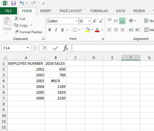
Step 1: Open the spreadsheet containing the #N/A value that you want to replace.
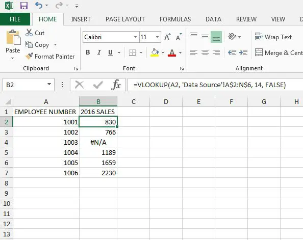
Step 2: Select a cell containing the formula that you want to change.
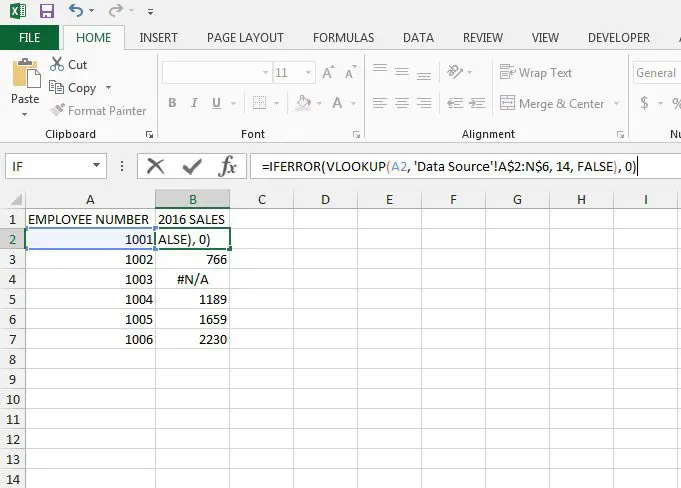
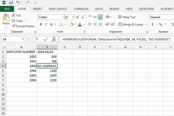
Step 3: Modify the existing VLOOKUP formula to include the IFERROR information.
This involves adding the phrase “IFERROR(” to the beginning of the formula, and the string “, 0)” to the end of the formula. For example, if your formula before was: =VLOOKUP(A2, ‘Data Source’!A$:N$6, 14, FALSE) Then you would modify it to be: =IFERROR(VLOOKUP(A2, ‘Data Source’!A$:N$6, 14, FALSE), 0)
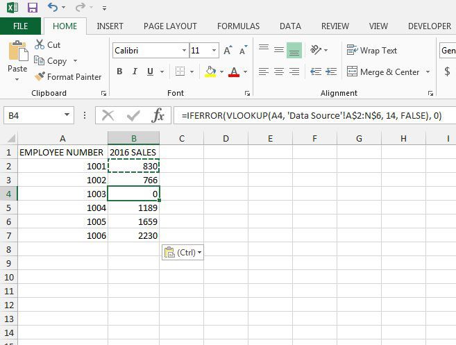
Step 4: Copy and paste the new formula into the cells where you want to display a “0” instead of #N/A.
Note that you can choose to display an string of characters that you would like. It doesn’t have to be a 0. For example, if you were using the VLOOKUP formula to insert an address, then you could make the formula =IFERROR(XX, YY:ZZ, AA, FALSE), “NO ADDRESS”). That would show the phrase “NO ADDRESS” instead of a 0 when Excel couldn’t find the data it wanted. Another helpful formula you can use is called CONCATENATE. This article will show you some ways that you can use that to combine data from multiple cells. You can also find out how to subtract in Excel with the help of another formula that can come in handy. Our guide continues below with additional discussion about how to make n/a 0 in Excel.
More Information on How to Switch VLOOKUP N/A to 0 in Excel
The IFERROR function is a very useful thing that you can add to the VLOOKUP function in Microsoft Excel. While, in a perfect world, all of your lookup value data will have a corresponding result based on the lookup values in your formula, if you use VLOOKUP enough you will eventually have a dataset with the occasional error value. Not only does that “n/a” value look bad, it can also be problematic if you are performing other functions on the data being pulled from the lookup range with the formula. By switching the value to a 0 you will ensure that users can still get totals if they include those values in sums, or if they are going to sort the columns or rows that contain the formula results. At the end of the tutorial in the previous section, we discussed replacing that 0 value with something else. While this article focuses specifically on changing the n/a value to a zero, using a custom value in that part of the formula can be really helpful when you are searching for errors in the middle of a large amount of data. The exact value that you can use will depend on your situation, but using something that really stands out, like a long text string of all capital letters, can make it much easier to identify problematic data in your spreadsheet.
Additional Sources
After receiving his Bachelor’s and Master’s degrees in Computer Science he spent several years working in IT management for small businesses. However, he now works full time writing content online and creating websites. His main writing topics include iPhones, Microsoft Office, Google Apps, Android, and Photoshop, but he has also written about many other tech topics as well. Read his full bio here.
You may opt out at any time. Read our Privacy Policy